Efficiently computing shared neighbors in graph

Problem background

Assume that we have a large graph containing many nodes and edges. For this graph, we need to compute the number of shared neighbors for each pair of nodes.
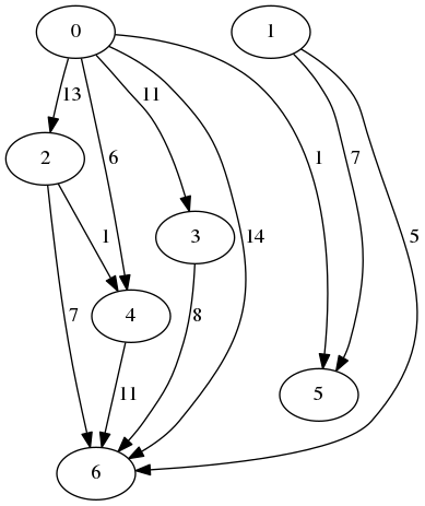
An instance example

For nodes 0 and 1, the result is 1 as the nodes share a single neighbor, which is node 2. For nodes 0 and 3, the result is 2 as both of them share nodes 2 and 4 as neighbors.

Naive solution

Assume that the input graph is represented in python networkx graphs. A trivial solution is to compute for all pairs the number of shared neighbors by neighbors intersection:

from itertools import combinations
import networkx as nx
from networkx.generators.random_graphs import gnp_random_graph

g: nx.Graph = gnp_random_graph(1000, 0.2)  # get a graph
shared_neighbors = {}
for node_1, node_2 in combinations(g.nodes, r=2):
    shared_neighbors[(node_1, node_2)] = (
        sum(1 for _ in nx.common_neighbors(g, node_1, node_2))
    )

This code is relatively trivial. The most expensive part of the code is getting the common neighbors. This code can be improved by computing shared neighbors faster.

Almost naive solution

A straight forward approach to optimize the performance is by indexing the neighbors beforehand in sets for each node. Using that, we don’t need to access the graph’s data structure, and avoid an expensive iteration.

from itertools import combinations
import networkx as nx
from networkx.generators.random_graphs import gnp_random_graph

g: nx.Graph = gnp_random_graph(1000, 0.2)  # get a graph
neighbors = {node: set(g.neighbors(node)) for node in g.nodes}
for node_1, node_2 in combinations(g.nodes, r=2):
    shared_neighbors[(node_1, node_2)] = (
        len(neighbors[node_1] & neighbors[node_2])
    )

The difference between the naive solution and the almost naive one is significant. On average, an example of 1000 nodes takes 90 seconds using the naive solution, and 3 seconds using the almost naive solution.

Now, can we do any better?

Optimizing using an adjacency matrix

Firstly, let us refresh our memory regarding how graphs are represented in a matrix.

Adjacency matrix

For undirected graphs, a common representation is an adjacency matrix. Denote by n the number of nodes, and denote by A a matrix of size n×n. The cell A[i,j]=1 if the nodes i and j are adjacent, and 0 otherwise.

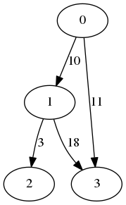
For example, the following graph:

Is represented by:

0101
1001
0001
1101
Adjacency matrix

Simply stating, each cell corresponds to a “potential” edge. If an edge connecting the ith node to a jth node exists in the graph, the cell value is 1, otherwise it is 0.

Intersection using multiplication

Let us also remember how matrix multiplication is performed. Given matrices A and B, both of size n×n, the (i,j) cell in the result is the sum of A[i,k]•B[k,j] over all values of k from 0 to n-1. Since our values are binarized, then A[i,k]•B[k,j] is either 0 or 1, where 1 means that A[i,k]=1 and B[k,j]=1, otherwise A[i,k]=0 or B[k,j]=0. Since in adjacency matrix A[i,j] indicates if i and j are adjacent, then the sum A[i,k]•B[k,j] over k is a counter of the shared neighbors of i and j.

Using the adjacency matrix above, set i=0 and j=1: A[0,0]•B[0,1]+A[0,1]•B[1,1]+A[0,2]•B[2,1]+A[0,3]B[3,1]=0+0+0+1=1, which corresponds to the single shared neighbor, node 3.

It is easy to see that if we multiply A by itself, each cell A[i,j] will contain the number of shared neighbors by i and j.

Now, let us look at a code that does exactly that:

A = nx.to_scipy_sparse_matrix(g)
A = (A**2).todok()

The code does three simple operations:

  • Convert the graph to adjacency matrix (a csr matrix in this case)
  • Multiply the adjacency matrix by itself
  • Convert the result matrix to dok matrix (a dictionary of keys representation)

The first two steps perform and the expected operations described for the optimizations. The last step is performed to make the comparison to the previous versions valid, as they yielded a dictionary that allowed access in O(1) to the intersection size.

On average, an example of 1000 nodes takes 3 seconds using the almost naive solution, and 0.8 seconds using the matrix-based solution. This is more than 3 times faster, and more than 100 times faster than the naive solution.

We won’t be going into two essential details of why matrix-based operations are faster, and representation by sparse matrix. Yet, we’ll assume for now that you already possess the processor-based intuition for it.

Summary

In this post, we presented a common problem of nodes close-neighborhood intersection. We presented how easy is it to get a working solution, and how to optimize by a factor of more than a 100 using a conversion of the representation to an adjacency matrix.

In general, many problems in graphs are easily translatable to matrix problems. When a performance issue arises in the original representation, a conversion to a matrix may ease the issue significantly.

Advertisement

Shortest path on sparse graphs

This post is an introduction to SciPy sparse graphs. It will present a variation of a known problem followed by a simple solution and implementation.

Problem background

We are given a directed acyclic graph (DAG) with dynamic edge costs. The graph is large in regard to nodes, it is expected to have millions of nodes. Additionally, the graph is expected to have very few edges, so the average degree is very small.

We need to construct a data structure that given two states, a source and a target, can figure our efficiently if there’s a path from the source to the target. In case it can, what would be the minimum cost of such path?

Our goal is to reduce the query time, where we expected the pairs of source and target to be uniformly picked.

For example, this representation could be of a system with many workflows, mostly independent, where each step in a workflow requires different effort to finish.

An instance example

The following graph is an example of such graph, where the edge labels represent the costs:

g

A query could be: Can 2 reach 6? The answer, in this case, is yes. The cost of reaching 6 from 2 is 7 (2→6). Please note the cost is the current cost. The path will always exist, but the edges price may change in the future.

Another query could be: Can 1 reach 2? The answer is no. No path from 1 to 2 exists. This answer will stay no forever, regardless any cost changes.

Problem characteristics

  1. Since the input is a graph, then any shortest-path algorithm could work. For example, Dijkstra’s algorithm. Yet, for any target node, the expected query time is at least as the number of nodes that can reach the target node.
  2. Remember that most states have very few transitions and that the graph is a DAG. This means that for a random pair of states, it is very unlikely that a path will exist.
  3. The edge costs are dynamic. This means that any solution that involves pre-calculation of the results will require re-calculation.
  4. The nodes set is large. Therefore, any exhaustive caching requires a lot of memory. If the number of nodes is 1,000,000 and each pair is represented using one bit, then cache would require ~125gb.

Solution guidelines

A straightforward approach would aim to reduce the number of shortest-path algorithm executions as most would yield “no path”. Therefore, some sort of method to predict paths existence is needed.

Assuming we want to initialize a cache, we would store in the cache the fact that i is reachable from rather than the distance itself since the prices are dynamic. In the case where the average degree is very low, we can expect most pairs to be false. Therefore, we can store only the pairs whose value is true. For example, in the case of 1M nodes and an average degree of 2, we expect <<1% to be true.

OK, let’s implement!

Sparse graph representation

A common representation of graphs is weighted adjacency matrix. Denote the matrix with A, and we say that the cost of the edge from i to price is A[i, jif the edge from i to j exists and 0 otherwise.

Adjacency matrix example

matrix_example

  0 1 2 3
0 0 10 0 11
1 0 0 3 18
2 0 0 0 0
3 0 0 0 0

In this example, has an edge to 1, so A[0, 1] = 10. 0 and 2 are not directly connected, so A[0, 2] = 0. The rows of 2 and 3 are all zeros since both are leaves, meaning their out degree is 0.

SciPy sparse matrix

We expect the majority of cells in the matrix to be 0. In this case, we can take advantage of a sparse matrix representation. The format which we will use is compressed sparse row (CSR), which supports efficient matrices multiplication. It requires O(num of edges) memory. Luckily, SciPy provides an implementation to the CSR matrix.

Given an input in a form of dictionary of edges to weight:

edges  = {
          (0, 1): 2,
          (0, 2): 3,
          (2, 3): 10,
          (3, 4): 1,
          (3, 5): 7
         }

We can transform it to a sparse matrix:

raw_weights = list(edges.values())
sources = [s for s, _ in edges.keys()]
targets = [t for _, t in edges.keys()]
n = max(sources + targets) + 1  # assume no isolated nodes
weights = csr_matrix((raw_weights, (sources, targets)), shape=(n, n))

This will result in our case to:

[[ 0 2 3 0 0 0]
 [ 0 0 0 0 0 0]
 [ 0 0 0 10 0 0]
 [ 0 0 0 0 1 7]
 [ 0 0 0 0 0 0]
 [ 0 0 0 0 0 0]]

Remember that the zeros in the matrix are “implicit” so don’t let the current representation mislead you regarding the memory consumption.

Computing reachable nodes

After representing the graph as a matrix, we can create a boolean adjacencies matrix. A boolean adjacencies matrix A is one where A[i, j] is true iff there is an edge from to j or i=j.

We will take advantage of the following propertyAk[i, j]=true iff exists a path from i to j of length k-1 or less. Let us look at an example:

matrix_powers

It is easy to create the adjacency matrix for this graph, and to follow its powers:

# A
[[ True True False False]
 [False True True False]
 [False False True True]
 [False False False True]]

# A2
[[ True True True False]
 [False True True True]
 [False False True True]
 [False False False True]]

# A3
[[ True True True True]
 [False True True True]
 [False False True True]
 [False False False True]]

Graph diameter

According to the graph diameter definition, any simple path is as long as the diameter. This means that if we know the graph diameter, we can easily resolve the reachable components by computing Adiameter.

Another property which is easy to notice is that the minimal k that satisfies Ak=Ak+1 is the graph diameter. Also, if k>diameter, then Ak+m=Ak for any positive m (since no new node will become reachable after walking all paths in the length of the diameter). Looking at A2, A4, A8,…, we can see that if two consecutive powers of A equal, we have reached the matrix that represents the reachable components.

All the values in the reachable components are either true or false. Also, for any Ak[i, j] that is true for some kAk+m[i, j] will be true for any positive m. This means that when we compare two powers of A, it is enough to compare the number of true values in the matrix.

Computing with adjacency matrix powers

Given an initial weights matrix, we can create the adjacencies matrix:

adjacency = (weights +
             sparse.diags(np.ones(weights.shape[0]), 0,
                          format='csr')).astype(bool)

The code takes the weights matrix and adds 1 to each value over the diagonal to ensure a positive value. Then it converts the matrix to a boolean one, so any cell with non-zero value turns into true.

Now, we can raise the matrix by powers of 2, until the number of true values does not change:

components = adjacency.copy()
previous_nnz = 0
while previous_nnz != components.nnz:
    previous_nnz = components.nnz
    components **= 2

The code compares the property nnz, which is the number of non-zero values, to the previous iteration count. Oofficially, nnz it is the number of explicit values stored, but in our case, it equals the number of non-zeros). When it reaches a stable matrix, the components matrix contains the reachable components, meaning that components[i, j]=true iff exists a path from i to j.

Querying nodes

Given a query with nodes i and j, two actions are required – check if i can reach j, and if so, compute the minimum cost of the path between them.

Reachability query

The format we’ve used for the components matrix is CSR, which is efficient for computing matrix powers, but, it does not allow constant time access for keys. Therefore, we would like to convert it into a more efficient representation, such as a set of pairs.

components = components.tocoo()
reachable_pairs = set(zip(components.row, components.col))

Firstly, we convert the CSR matrix into a coordinates matrix, which is more iteration friendly. The row and col attributes are arrays containing the coordinates of the true stored values.

For example, if the matrix is:

[[False True]
 [True False]]

Then:

row = [0, 1]
col = [1, 0]

This results with

reachable_pairs = {(0, 1), (1, 0)}

Path cost querying

Now that we have a quick way to check if a path exists, we can execute the dijkstra algorithm on the weights matrix:

if (source, target) in reachable_pairs:
    distances = dijkstra(weights, indices=[source])
    distance = distances[0, target]
else:
    distance = np.inf

The call to dijkstra returns a costs vector from source to all the nodes in the graph. In our case we expect the vast majority to be infinity.

Summary

In this post, we’ve seen one approach to efficiently handle shortest path problem on very sparse graphs. We chose a representation based on sparse adjacency matrix and pre-computed all the connected components.

I will mention the benchmarks, ~500 times faster on 100K nodes with an average degree of 2, but please note that this is not enough to generalize. The main reason is that the problem introduced is too naive – no prior knowledge of the components and queries with a uniform distribution over the nodes. This is usually not the case in real life problems. Information about the components, or a distribution with a higher expectation of positive hits, might have changed the approach.

There are other approaches to optimize, yet, it is very encouraging to know how simple can solutions can be, ~20 lines of code, and very lightweight. It can be useful in many cases to translate problems into classic problems in graphs and take advantage of the existing theory and implementations. This is also true even when large amounts of data are involved.

Field initializers and base constructors order

In this post we’ll explore what happens behind the scenes when we place code in field initializer compared to constructor body.

Field initializer and constructor

We’ll start from a simple example:

public class MyClass
{
private static int index = 1;

public int x = index++;
public int y;

public MyClass()
{
y = index++;
}
}

The result here is very intuitive, this code:

var instance = new MyClass();
Console.WriteLine("x = " + instance.x);
Console.WriteLine("y = " + instance.y);

Will output:
image

So far there’s no surprise, the field initializers code is performed prior to code of the explicit constructor.

Field initializer and base constructor

Let’s observe the next code:

public class Base
{
protected static int index = 1;

public int w = index++;
public int x;

public Base()
{
x = index++;
}
}

public class Derived : Base
{
public int y = index++;
public int z;

public Derived()
{
z = index++;
}
}

There are two outputs which one may expect:

  • The base class fields will be initialized first and the derived ones will be initialized afterwards.
  • The field y, which has a field initializer will be initialized first, then the base fields and lastly the derived constructor will be called.

What actually happens?

var instance = new Derived();
Console.WriteLine("Base.w = " + instance.w);
Console.WriteLine("Base.x = " + instance.x);
Console.WriteLine("Derived.y = " + instance.y);
Console.WriteLine("Derived.z = " + instance.z);

Outputs:
image

We can clearly see that the derived field initializer is called first, prior to the base constructor.

Why it happens?

Looking at the disassembled IL we can see that the field initializers code is placed at the beginning of the constructor code, prior to the base constructor call:

.method public hidebysig specialname rtspecialname 
instance void .ctor() cil managed
{
// Code size 48 (0x30)
.maxstack 8
IL_0000: ldarg.0
IL_0001: ldsfld int32 ConsoleApplication1.Base::index
IL_0006: dup
IL_0007: ldc.i4.1
IL_0008: add
IL_0009: stsfld int32 ConsoleApplication1.Base::index
IL_000e: stfld int32 ConsoleApplication1.Derived::y
IL_0013: ldarg.0
IL_0014: call instance void ConsoleApplication1.Base::.ctor()
IL_0019: nop
IL_001a: nop
IL_001b: ldarg.0
IL_001c: ldsfld int32 ConsoleApplication1.Base::index
IL_0021: dup
IL_0022: ldc.i4.1
IL_0023: add
IL_0024: stsfld int32 ConsoleApplication1.Base::index
IL_0029: stfld int32 ConsoleApplication1.Derived::z
IL_002e: nop
IL_002f: ret
} // end of method Derived::.ctor

We can see, obviously, that the compiler is protecting us from doing silly mistakes like accessing base fields before they’re initialized:

public class Base
{
protected int baseField = 100;
}

public class Derived : Base
{
public int x = baseField;
}

Leads to a compilation error, while this code works perfectly:

public class Derived : Base
{
public int x;

public Derived()
{
x = baseField;
}
}

Does it really matter?

Understanding our code

I guess that in almost all cases this will not cause noticeable difference. It will however make a difference when we’re depending on that order, or, when the field initializers call methods that depend on side effects. So for start it’s important that we understand how our code works.

Make use of it

The next thing we can do is to use the field initializers as a hack to precede base constructors code. For example, if we have this 3rd party logger:

public class MyLogger
{
public MyLogger()
{
if (!Directory.Exists(@"C:\Logs"))
{
throw new InvalidOperationException("Can't start logs");
}

File.WriteAllText(@"C:\Logs\Session.log", "Initialized");
}
}

And we want to change it’s behavior without rerouting all it’s methods (of course this is not the only way), we can initialize a dummy field with method call that creates the directory:

public class MyLoggerHack : MyLogger
{
private bool dummy = CreateDirectory();

private static bool CreateDirectory()
{
if (!Directory.Exists(@"C:\Logs"))
{
Directory.CreateDirectory(@"C:\Logs");
}

return true;
}
}

So using this hack, we can “add” new code to the beginning of an existing call constructor without actually changing the original class.

Implementing switch fall through in C#

In this post I’ll introduce a less known feature of the C# language – the goto expression.

In general, we know that it is not a great idea to use goto statements in code since it raises significantly the chance of ending up with spaghetti code. Reading and understanding of spaghetti code is way more difficult and therefore its maintenance is expensive.

The case we are going to deal with is goto inside single switch statement. It results that all the labels are local – this case is usually much easier to track than distanced labels. The goto statements enable us to implement the fall through capability which is not supported out of the box in C#.

Switch fall through

In C# implicit fall through between cases in C# is not allowed. The reason for disallowing it is simple – implicit fall through is likely to cause bugs since forgetting to place a break is very common mistake. C# switch statements require each case to end with an explicit end point or a sure “never ending” code. End points are explicit expressions that transfers the execution out of the case block, these can be break, goto, throw and return. A never ending code is code that we know for sure during compilation it is never going to exit the block, such as a while loop whose condition is true.

According to these requirements it is clear that implicit fall through is not supported since we provide explicit instruction about how each case ends.

goto statements

goto in C# is simple and consistent with most languages like C and C++. It is based on labels, which are defined in the code by ‘label-name:’ followed by a C# statement. In order to jump to a label we use the goto statement with the label – ‘goto label-name;’’.

This is a simple implementation of a loop with based on goto.

public void GotoBasedLoop()
{
int times = 3;
int i = 0;
start:
if (i >= times)
{
goto end;
}

Console.WriteLine(i);
i++;
goto start;

end:
return;
}

goto statements in switch

As we’ve seen – each case must have an end point or a promise it never ends. It leads that using naïve usage of gotos we can implement the fall through – we place a label at the beginning of every case and use a goto at the end of every case we want to redirect.

Luckily, for this case C# provides a labels like behavior that simplifies the usage. Each case can be redirected to other case using a simple syntax – goto case ‘constant’ or goto default. Using this syntax we can avoid a duplicate label for fall through.

This usage can be exampled by a simple code that “counts” asterisks:

static int GetLength(string s)
{
int x = 0;

switch (s)
{
case "*":
x++;
break;
case "**":
x++;
goto case "*";
case "***":
x++;
goto case "**";
}

return x;
}

As can be seen, each case is redirected to a different case using the built in mechanism.

Summary

Fall through is probably not the most common feature that developers look for. Since implicit fall through is more likely to cause bugs than simplify coding the C# designers decided to leave it out of the language. For those cases where we want to keep things simple – avoid extracting code to a method just for reuse or instead to create code duplication – we can use the simple solution of redirecting cases using goto.