This post is an introduction to SciPy sparse graphs. It will present a variation of a known problem followed by a simple solution and implementation.

Problem background

We are given a directed acyclic graph (DAG) with dynamic edge costs. The graph is large in regard to nodes, it is expected to have millions of nodes. Additionally, the graph is expected to have very few edges, so the average degree is very small.

We need to construct a data structure that given two states, a source and a target, can figure our efficiently if there’s a path from the source to the target. In case it can, what would be the minimum cost of such path?

Our goal is to reduce the query time, where we expected the pairs of source and target to be uniformly picked.

For example, this representation could be of a system with many workflows, mostly independent, where each step in a workflow requires different effort to finish.

An instance example

The following graph is an example of such graph, where the edge labels represent the costs:

A query could be: Can 2 reach 6? The answer, in this case, is yes. The cost of reaching 6 from 2 is 7 (2→6). Please note the cost is the current cost. The path will always exist, but the edges price may change in the future.

Another query could be: Can 1 reach 2? The answer is no. No path from 1 to 2 exists. This answer will stay no forever, regardless any cost changes.

Problem characteristics

1. Since the input is a graph, then any shortest-path algorithm could work. For example, Dijkstra’s algorithm. Yet, for any target node, the expected query time is at least as the number of nodes that can reach the target node.
2. Remember that most states have very few transitions and that the graph is a DAG. This means that for a random pair of states, it is very unlikely that a path will exist.
3. The edge costs are dynamic. This means that any solution that involves pre-calculation of the results will require re-calculation.
4. The nodes set is large. Therefore, any exhaustive caching requires a lot of memory. If the number of nodes is 1,000,000 and each pair is represented using one bit, then cache would require ~125gb.

Solution guidelines

A straightforward approach would aim to reduce the number of shortest-path algorithm executions as most would yield “no path”. Therefore, some sort of method to predict paths existence is needed.

Assuming we want to initialize a cache, we would store in the cache the fact that i is reachable from j rather than the distance itself since the prices are dynamic. In the case where the average degree is very low, we can expect most pairs to be false. Therefore, we can store only the pairs whose value is true. For example, in the case of 1M nodes and an average degree of 2, we expect <<1% to be true.

OK, let’s implement!

Sparse graph representation

A common representation of graphs is weighted adjacency matrix. Denote the matrix with A, and we say that the cost of the edge from i to j price is A[i, j] if the edge from i to j exists and 0 otherwise.

Adjacency matrix example

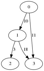
	0	1	2	3
0	0	10	0	11
1	0	0	3	18
2	0	0	0	0
3	0	0	0	0

In this example, 0 has an edge to 1, so A[0, 1] = 10. 0 and 2 are not directly connected, so A[0, 2] = 0. The rows of 2 and 3 are all zeros since both are leaves, meaning their out degree is 0.

SciPy sparse matrix

We expect the majority of cells in the matrix to be 0. In this case, we can take advantage of a sparse matrix representation. The format which we will use is compressed sparse row (CSR), which supports efficient matrices multiplication. It requires O(num of edges) memory. Luckily, SciPy provides an implementation to the CSR matrix.

Given an input in a form of dictionary of edges to weight:

edges  = {
          (0, 1): 2,
          (0, 2): 3,
          (2, 3): 10,
          (3, 4): 1,
          (3, 5): 7
         }

We can transform it to a sparse matrix:

raw_weights = list(edges.values())
sources = [s for s, _ in edges.keys()]
targets = [t for _, t in edges.keys()]
n = max(sources + targets) + 1  # assume no isolated nodes
weights = csr_matrix((raw_weights, (sources, targets)), shape=(n, n))

This will result in our case to:

[[ 0 2 3 0 0 0]
 [ 0 0 0 0 0 0]
 [ 0 0 0 10 0 0]
 [ 0 0 0 0 1 7]
 [ 0 0 0 0 0 0]
 [ 0 0 0 0 0 0]]

Remember that the zeros in the matrix are “implicit” so don’t let the current representation mislead you regarding the memory consumption.

Computing reachable nodes

After representing the graph as a matrix, we can create a boolean adjacencies matrix. A boolean adjacencies matrix A is one where A[i, j] is true iff there is an edge from i to j or i=j.

We will take advantage of the following property: A^k[i, j]=true iff exists a path from i to j of length k-1 or less. Let us look at an example:

It is easy to create the adjacency matrix for this graph, and to follow its powers:

# A
[[ True True False False]
 [False True True False]
 [False False True True]
 [False False False True]]

# A2
[[ True True True False]
 [False True True True]
 [False False True True]
 [False False False True]]

# A3
[[ True True True True]
 [False True True True]
 [False False True True]
 [False False False True]]

Graph diameter

According to the graph diameter definition, any simple path is as long as the diameter. This means that if we know the graph diameter, we can easily resolve the reachable components by computing A^diameter.

Another property which is easy to notice is that the minimal k that satisfies A^k=A^k+1 is the graph diameter. Also, if k>diameter, then A^k+m=A^k for any positive m (since no new node will become reachable after walking all paths in the length of the diameter). Looking at A², A⁴, A⁸,…, we can see that if two consecutive powers of A equal, we have reached the matrix that represents the reachable components.

All the values in the reachable components are either true or false. Also, for any A^k[i, j] that is true for some k, A^k+m[i, j] will be true for any positive m. This means that when we compare two powers of A, it is enough to compare the number of true values in the matrix.

Computing with adjacency matrix powers

Given an initial weights matrix, we can create the adjacencies matrix:

adjacency = (weights +
             sparse.diags(np.ones(weights.shape[0]), 0,
                          format='csr')).astype(bool)

The code takes the weights matrix and adds 1 to each value over the diagonal to ensure a positive value. Then it converts the matrix to a boolean one, so any cell with non-zero value turns into true.

Now, we can raise the matrix by powers of 2, until the number of true values does not change:

components = adjacency.copy()
previous_nnz = 0
while previous_nnz != components.nnz:
    previous_nnz = components.nnz
    components **= 2

The code compares the property nnz, which is the number of non-zero values, to the previous iteration count. Oofficially, nnz it is the number of explicit values stored, but in our case, it equals the number of non-zeros). When it reaches a stable matrix, the components matrix contains the reachable components, meaning that components[i, j]=true iff exists a path from i to j.

Querying nodes

Given a query with nodes i and j, two actions are required – check if i can reach j, and if so, compute the minimum cost of the path between them.

Reachability query

The format we’ve used for the components matrix is CSR, which is efficient for computing matrix powers, but, it does not allow constant time access for keys. Therefore, we would like to convert it into a more efficient representation, such as a set of pairs.

components = components.tocoo()
reachable_pairs = set(zip(components.row, components.col))

Firstly, we convert the CSR matrix into a coordinates matrix, which is more iteration friendly. The row and col attributes are arrays containing the coordinates of the true stored values.

For example, if the matrix is:

[[False True]
 [True False]]

Then:

row = [0, 1]
col = [1, 0]

This results with

reachable_pairs = {(0, 1), (1, 0)}

Path cost querying

Now that we have a quick way to check if a path exists, we can execute the dijkstra algorithm on the weights matrix:

if (source, target) in reachable_pairs:
    distances = dijkstra(weights, indices=[source])
    distance = distances[0, target]
else:
    distance = np.inf

The call to dijkstra returns a costs vector from source to all the nodes in the graph. In our case we expect the vast majority to be infinity.

Summary

In this post, we’ve seen one approach to efficiently handle shortest path problem on very sparse graphs. We chose a representation based on sparse adjacency matrix and pre-computed all the connected components.

I will mention the benchmarks, ~500 times faster on 100K nodes with an average degree of 2, but please note that this is not enough to generalize. The main reason is that the problem introduced is too naive – no prior knowledge of the components and queries with a uniform distribution over the nodes. This is usually not the case in real life problems. Information about the components, or a distribution with a higher expectation of positive hits, might have changed the approach.

There are other approaches to optimize, yet, it is very encouraging to know how simple can solutions can be, ~20 lines of code, and very lightweight. It can be useful in many cases to translate problems into classic problems in graphs and take advantage of the existing theory and implementations. This is also true even when large amounts of data are involved.